A Primer on Measure Theory

The story of one of the best PhD theses of all time

This is a standalone post, although in some ways it acts as a bridge between two posts that I have already written and another that I intend to write.

Specifically, a recurring theme in this post is that we will study under what circumstances we might exchange a limit and an integral. If you are wondering why that might be something anyone would care about, my last two articles on functional analysis provide that motivation.

Why Functional Analysis?

WTF is a Hilbert Space?

On the other hand, the tools we build now will be very useful when I finally write about how one can build up quantum mechanics via functional analysis.

---

This is the story of Henri Lebesgue’s PhD thesis, published in 1902, which single-handedly revolutionized integration and paved the road for the development of functional analysis, modern probability theory, ergodic theory, and much more.

It was, in short, one of the greatest PhD theses ever written.

Before we get into Lebesgue’s clever solution, let’s talk about the main problem: let’s say that you want to consider a limit

\(\lim_{n\rightarrow\infty}\int_a^b f_n(x) \ \text{d}x.\)

Under what circumstances can you exchange the order and instead consider

\(\int_a^b \lim_{n\rightarrow\infty} f_n(x) \ \text{d}x?\)

(If you are wondering why you might want to do that, I refer you again to the previous two functional analysis posts.)

There are various obstructions to being able to exchange the order, but let’s consider one that you might not expect: if we are working with the Riemann integral, the second integral might not even be defined. Let’s illustrate this with a toy example.

Define 1_ℤ(x) to be 1 if x is an integer, and 0 otherwise. Then define f_n(x)=1_ℤ(2ⁿx)—this is 1 if x is an integer multiple of 2^-n, and 0 otherwise. Because each of these functions is 0 other than at some discrete set of points, it is easy to see that

\(\int_0^1 f_n(x) \ \text{d}x = 0\)

for all n, which means that the limit is also 0. Is this the same as

\(\int_0^1 \lim_{n\rightarrow\infty}f_n(x) \ \text{d}x?\)

Well, in the pointwise limit, these functions converge to

\(f(x) = \begin{cases} 1 & \text{if } x=k/2^n \text{, $k,n$ integers} \\ 0 & \text{otherwise}. \end{cases}\)

Here’s the problem: this isn’t Riemann integrable!

Let’s quickly remind ourselves how the Riemann integral works. To define the integral of f over an interval [a, b], you consider partitions of the interval: we choose points a=x₀<x₁<x₂<…<x_n+1=b, where we ask that x_i+1-x_i<Δx for some real number Δx>0. We then define the Riemann sum

\(\sum_{i=0}^n f(x_i^*)(x_{i+1}-x_i),\)

where x_i≤x_i*≤x_i+1 is an arbitrarily chosen real number. Geometrically, we are calculating the (signed) areas of rectangles with x_i<x<x_i+1 and 0<y<f(x_i*) to approximate the area under the curve.

A sequence of Riemann sums approximating an integral, with Δx getting smaller and smaller.

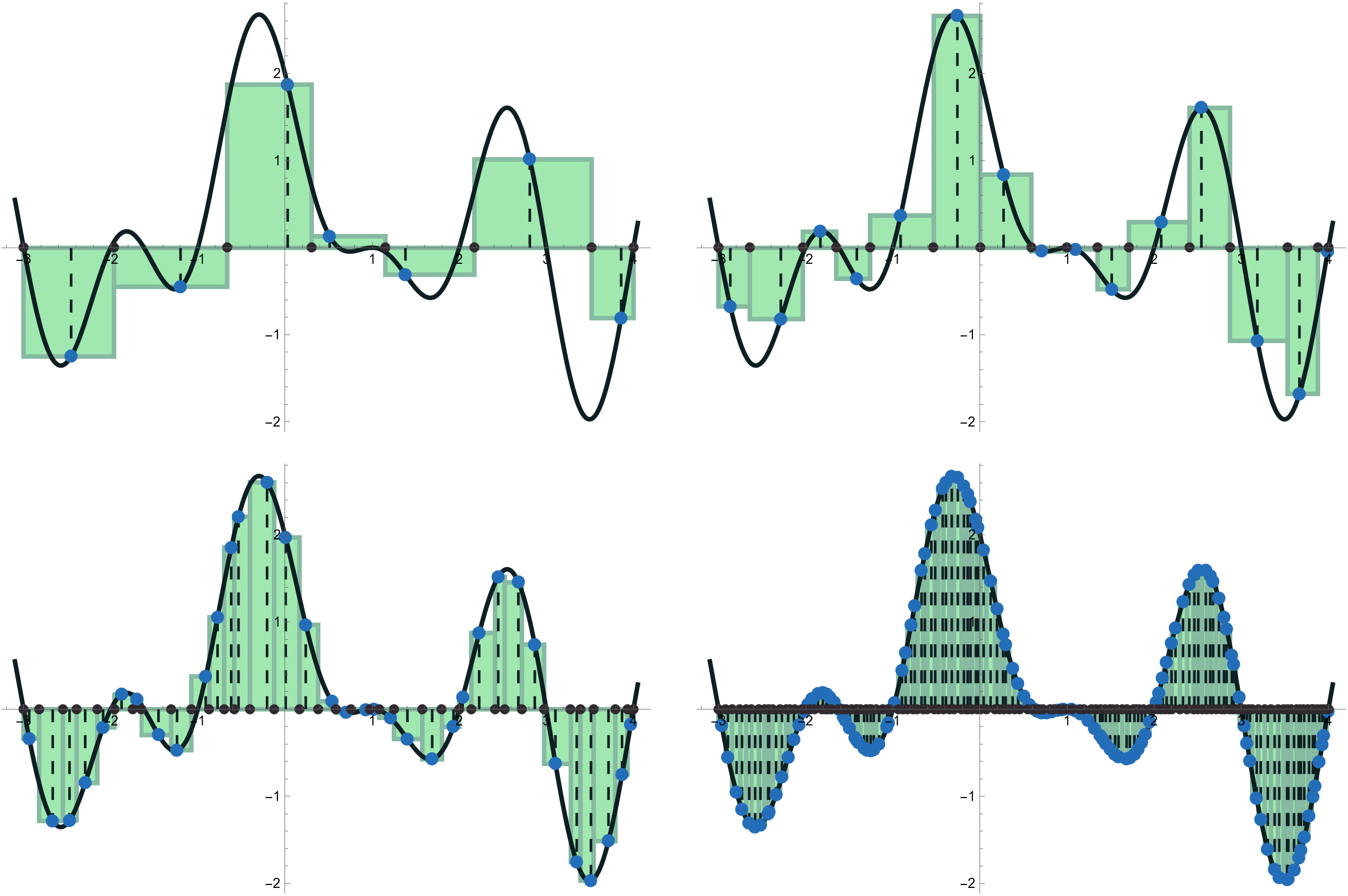
Finally, we take the limit as Δx→0. As long as the limit

\(\lim_{\Delta x\rightarrow 0}\sum_{i=0}^n f(x_i^*)(x_{i+1}-x_i)\)

exists and doesn’t depend on the choices of x_i*, then we say that f is Riemann-integrable and this limit is the integral of f over [a,b].

Now, let’s get back to our function. Unfortunately, the Riemann sums are extremely sensitive to the choice of x_i*! Observe that for any partition, we can always choose the x_i* such that f(x_i*)=1 for all i, that it is 0 for all i, or anything in between. (This is because between any two real numbers, there are always reals of the form k/2ⁿ and reals not of that form.)

Uh oh!

Now, you might protest at this juncture that the problem is that we are taking a very pathological example—surely, continuous/smooth/analytic functions wouldn’t betray us like this? I’m afraid that they can—indeed, you can find a sequence of polynomials p_n such that

\(\int_0^1 p_n(x) \ \text{d}x =0\)

for all n, but the pointwise limit of these polynomials is not Riemann-integrable.

So, what to do? Lebesgue came up with an ingenious solution: we need to come up with a better type of integration.

His first step was to introduce the notions of a σ-algebra and a measure. We’ll define what a σ-algebra is in a moment—for now, just think of it as a collection of subsets of some set X, and we’ll work out what properties it has to have as we go—and jump directly into working out what a measure is.

---

Definition: Let Σ be a σ-algebra of a set X. A measure on Σ is a function μ: Σ→[0,∞] satisfying the following properties:

1. μ(∅)=0 (here, ∅ denotes the empty set—i.e., the set that doesn’t contain anything), and

2. for any disjoint (countable) collection of sets E₁, E₂,… in Σ, the measure of their union is the sum of their measures:

   \(\mu\left(\bigcup_{i=1}^\infty E_i\right)=\sum_{i=1}^\infty \mu(E_i).\)

---

A measure does exactly what it says on the tin: it measures the size of subsets. Here’s an example: take any set X whatsoever, take Σ to be the full collection of subsets of X, and define μ(E) to be the number of elements in E.¹ This is known as the counting measure, which is fitting.

Here’s another example: take any set X, take Σ to be all subsets of X, choose any particular element in X, and define μ(E) to be 1 if E contains x, and 0 otherwise. This is known as the Dirac measure.²

Before we go further, let’s work out what a σ-algebra is, after all—that is, what properties do we need our collection of subsets to have for the definition of a measure to make sense?

Well, obviously, the empty set must be included—otherwise, the first property is nonsense. Secondly, if E₁, E₂,… are all valid subsets, their union should also be a valid subset—otherwise, the second property is nonsense.

There is one last property that it would be good to have. Suppose that E is a subset of F, both of which are valid subsets. Let G be the complement of E in F—the collection of all elements that are in F but not in E. I would like to say that μ(E)+μ(G)=μ(F)… but that might not make sense, because G might not be a valid subset unless we specifically request that it is!

Putting everything together, we have the definition that we need.

---

Definition: Let X be a set. A σ-algebra over X is a collection of subsets Σ such that

1. ∅ is in Σ,

2. if E₁, E₂,… are all in Σ, then so is their (countable) union, and

3. if E is in Σ, then so is the complement X\E.

---

From these, you can prove that the σ-algebra is also closed under (countable) intersections (this is just an application of De Morgan’s laws), and from that you can show that we can take complements not just in X, but inside any subset of the σ-algebra.

Here’s a more interesting example of a σ-algebra than the ones that I have included so far. Start with the collection of all open subsets of the real numbers—that is, all unions of open intervals (a,b). This is not a σ-algebra because it isn’t closed under complements. That’s fine: add on all closed sets (that is, complements of open sets) to this collection.

This is no longer closed under (countable) unions—i.e., it contains (0,1) and [1,2], but not their union, (0,2]. That’s fine: throw on all such (countable) unions. Now it isn’t closed under complements! That’s fine…

Keep doing this, ad infinitum. The claim is that you do get a σ-algebra this way—it is called the Borel algebra—but it is not the full collection of subsets of the real numbers.³

(If one is familiar with topological spaces, or at least metric spaces, then I will note that, yes, it is possible to define a corresponding Borel algebra by starting with open sets and adding sets as necessary, in the same way.)

Here’s an alternative way to build this σ-algebra, which is a little easier to work with: start with the collection of half-open intervals (a,b]. Close it under (countable) unions, then close it under complements, then close it under (countable) unions… Continue ad infinitum, and you’ll get the exact same thing as before. (One way to see this: any open interval is a countable union of such half-open intervals.)

Let’s define a measure on this σ-algebra, as follows: first, define μ((a,b])=b-a. Observe that this satisfies the properties of a measure: the empty set gets measure 0, and since

\(\begin{align*} c-a&=\mu\left((a,c]\right)=\mu\left((a,b] \cup (b,c]\right) \\ &= (b-a)+(c-b) = \mu\left((a,b]\right) + \mu\left((b,c]\right), \end{align*}\)

we get that the measure of the disjoint (countable) union is the sum of the measures. Of course, the collection of half-open intervals isn’t a σ-algebra, but that’s fine! We can simply extend this definition to the entire σ-algebra recursively. Say we already know how to define the measure of E₁ and E₂, which are two disjoint sets. Then we can define

\(\mu(E_1\cup E_2):=\mu(E_1)+\mu(E_2).\)

More generally, we do this with a (countably) infinite number of sets E₁, E₂,… Similarly, if E₂ is a subset of E₁ and E₃=E₁\E₂, then we will define μ(E₃)=μ(E₁)-μ(E₂). One checks that this produces a unique measure on the entire Borel algebra, known as the Lebesgue measure.⁴

How should we think about this measure? The measure of a single interval is just its length, and all other sets are obtained by extending that definition. One can also observe that

\(\int_a^b 1 \ \text{d}x = \mu([b,a]).\)

This suggests that we might try to define our integral for an arbitrary set E in the Borel algebra as

\(\int_E 1 \ \text{d}x = \mu(E).\)

In fact, that is exactly what we will do! We will, of course, then have to figure out how to define the integral of some function other than 1.

But, before we get into any of those details, let’s observe that this definition already fixes the problem that we encountered at the beginning! Here’s how: let D be the subset of elements in [0,1] of the form k/2ⁿ. Then f is the indicator function 1_D for D—that is, 1_D(x)=1 if x is in D and 0 otherwise. And so we define

\(\int_0^1 f(x) \ \text{d}x=\int_0^1 1_D \ \text{d}x=\mu(D).\)

What is the measure of D? Easy: the measure of a single point is 0 (since μ([x,x])=x-x=0), and D is a disjoint, countable union of points. It has measure exactly zero, as expected!

We can actually do this completely generally: take any measure μ on any σ-algebra on a set X—there is absolutely nothing special about the real numbers here—and define

\(\int_X 1_D \ \text{d}\mu := \mu(D),\)

where 1_D is the indicator function for D, where D is any subset in our algebra.

How can we proceed beyond this? Here’s an idea.

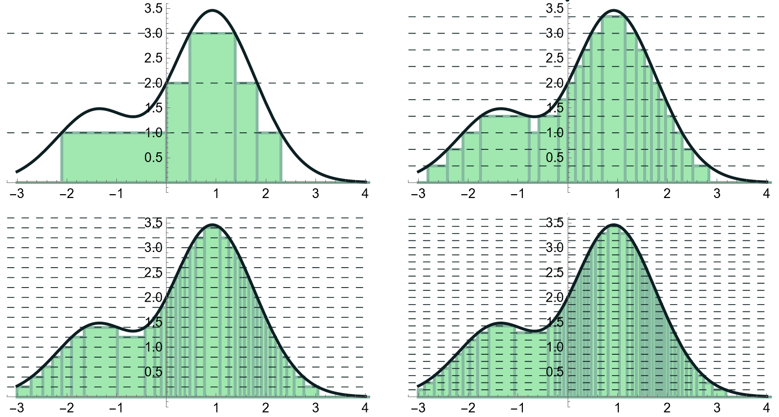
What I have done is set up a sequence of Riemann-like sums for a function, but in a somewhat different way: instead of splitting up the domain as we did before, I have split up the codomain. So, I might take two y-values y₁<y₂, consider all points where f is somewhere between those two values, and estimate f(x)=y₁ for any such points.

In other words, I took an interval (y₁,y₂), considered the pre-image f^-1((y₁,y₂)), and then estimated f as being constant along that pre-image. Putting everything together,

\(\begin{align*} \int_a^b f(x) \ \text{d}x &\approx \sum_{i=0}^n y_i\mu\left(f^{-1}((y_i,y_{i+1})\right) \\ &= \sum_{i=0}^n y_i \int_a^b 1_{f^{-1}((y_i,y_{i+1})} \ \text{d}\mu, \end{align*}\)

where y₀<y₁<y₂<…<y_n is our partition of the codomain.

Ah ha! So to get approximations, it is sufficient to consider simple functions: functions of the form

\(s(x)=\sum_{i=0}^n c_i 1_{D_i}(x),\)

where the sets D_i are in our σ-algebra, and the c_i’s are real numbers.⁵ It is entirely obvious how to define the integral of any such function:

\(\int_X s \ \text{d}\mu = \sum_{i=0}^n c_i \mu(D_i).\)

Now that we know how to get our approximations, all that remains is how to relate it back to the original function. For the real line, we could do a Riemann-style argument of taking a limit of ever finer partitions. But it isn’t so clear how to make that work for other spaces, whereas so far our theory of integration has been completely general.

Thankfully, there is a straightforward solution. First, observe that it is sufficient to consider functions f≥0. If not, we note that f=max(f,0)-max(-f,0), and so we can define

\(\int f \ \text{d}\mu = \int \max(f,0) \ \text{d}\mu-\int \max(-f,0) \ \text{d}\mu.\)

Then, consider the set S_f consisting of all simple functions s such that f(x)≥s(x) for all x. We then define

\(\int_X f \ \text{d}\mu := \sup_{s\in S_f} \int_X s \ \text{d}\mu.\)

And that’s it!

Under what circumstances will this definition make sense? As per our observation that we could look at the pre-images, we need it to be the case that if D is a subset in our algebra, then so is f^-1(D). (Otherwise, how would we define μ(f^-1(D))?)

This leads to our final definition.

---

Definition: Let Σ₁, Σ₂ be σ-algebras on two sets X, Y. A function f: X→Y is measurable if for all E in Σ₂, f^-1(E) is in Σ₁. (In the special case where Y=ℝ, we shall always assume that we are using the Lebesgue measure.)

Given a measure μ on Σ, for any measurable function f: X→ℝ, we define the integral of f with respect to μ as we did above. The function is integrable if

\(\int_X f \ \text{d}\mu\)

is defined and finite.

---

Now, there are various things you want to prove here. You want to prove that if f≥0, then so is its integral. You want to prove that the integral is linear (i.e., the integral of a sum is the sum of the integrals, and you can freely pull out constants). And so on. But this is just meant to give the essentials of measure theory, so we will skip all of that.

Instead, let’s examine what this integral actually is for various cases.

For the Lebesgue measure, the corresponding integral is essentially the same as the Riemann integral except that a wider array of functions now have definable integrals. (That is, on any interval [a,b], all Riemann-integrable functions are Lebesgue-integrable, and the values of the integrals match.) So we don’t mess up any of our older integration theory—we just get a better framework in which to consider it.

But that is not all, because we can consider measures other than the Lebesgue one!

For instance, take the counting measure. What is the corresponding integral? If you run through the details, you will discover that

\(\int_X f \ \text{d}\mu = \sum_{x\in X} f(x).\)

Many calculus classes introduce the integral as being an analog of an infinite sum. But from the measure-theoretic point of view, it is actually the opposite: infinite sums are particular examples of integrals! This has a very nice consequence: all general-purpose theorems (such as various convergence tests) that we prove about integrals will automatically apply to infinite series.

Another example: take the Dirac measure corresponding to a particular point x₀. The corresponding integral is also very simple:

\(\int_X f \ \text{d}\mu = f(x_0).\)

Physicists have this notion of a Dirac delta function δ with the property that

\(\int_{-\infty}^\infty f(x) \delta(x) \ \text{d}x = f(0).\)

Now, no such real-valued function on the real line exists. (And, to be fair, physicists don’t pretend otherwise—they just use it as a useful fiction for computations.) But one way that you can formally define the Dirac delta function is to instead use the Dirac measure, which doesn’t just exist—it’s actually quite simple.⁶

Do we get any other benefits from the framework of measure theory aside from greater generality and better behavior with respect to limits? Yes, quite a few actually.

To start, measure theory gives some very powerful results about when it is possible to exchange limits and integrals. Here’s probably the most famous and most commonly used one.

---

Theorem: (The Dominated Convergence Theorem) Let μ be a measure on a set X, and let f_n be a sequence of measurable functions X→ℝ that converge pointwise to a function f. Suppose further that there exists some integrable function g such that |f_n(x)|≤g(x) for all n and x. Then f_n and f are all integrable and

\(\lim_{n\rightarrow\infty}\int_X f_n \ \text{d}\mu = \int_X f \ \text{d}\mu.\)

---

Here’s another reason why it is so useful: measure theory is the natural setting in which to study probability. To see why, let’s recite Kolmogorov’s probability axioms. Let X be the sample space: you can think of it as the space of all possible outcomes/measurements. Let Σ be the space of all events, which are sets of outcomes. (You can think of an event E as saying that “x happens, or y happens, or…” where x,y are elements of X.) We are interested in assigning a probability P(E) to each event, and this must work as follows:

1. P(E)≥0 (probability should be non-negative),

2. P(X)=1 (the probability of literally any possible outcome occurring should be 100%), and

3. if E₁, E₂,… are disjoint events, then

   \(P\left(\bigcup_{i=1}^\infty E_i\right) = \sum_{i=1}^\infty P(E_i).\)

Do you see it? These are just the conditions for being a measure, plus the restriction that the measure of the entire space is 1! So, a simpler way to state Kolmogorov’s axioms is that probability P should be a probability measure on the space of possible outcomes X—that is, P(X)=1. And so, examples of probability measures include:

• μ_L/(b-a) on any interval [a,b], where μ_L is the Lebesgue measure. (This is what is meant when we talk about choosing a number a≤x≤b uniformly at random.)

• μ_C/n on any set X of n elements, where μ_C is the counting measure. (This is what is meant when we talk about choosing one of n elements uniformly at random.)

• μ_p on any set X with an element p, where μ_p is the Dirac measure. (I’ll let you think about how to interpret this in terms of probability.)

And all of this is just the beginning! We could talk about things like Haar measures, or the Hausdorff measure, or the measures associated to self-adjoint operators on a Hilbert space—there are countless ways in which measure theory ends up useful. But I think it is best to wrap up here.

1. We don’t care about cardinality here: if there are infinitely many elements, we simply write μ(E)=∞, regardless of whether the set is countable or uncountable.

2. Yes, this is related to the Dirac delta function—we’ll get to that!

3. Okay, technically what I have just said is only true if you subscribe to the Axiom of Choice, or at least some slightly weaker version of Choice. However, there exists a model of ZF (without Choice) in which every subset is, indeed, Borel!

4. Strictly speaking, this isn’t quite correct: the Lebesgue measure is what one obtains by completing this measure. Specifically, for every measure-zero set, we add its subsets to the Borel algebra (and give them measure zero). But these are technical details that we can ignore on a first reading.

5. Complex numbers also work, although we won’t need that here.

6. Unfortunately, there are various operations that physicists like doing with the Dirac delta function that are not so elegant to describe in terms of measures—differentiation and the Laplace transform come to mind. I personally prefer formalizing the Dirac delta in a different way, but that is a topic for another time.