Why Functional Analysis?

An introduction to the field that enforced rigor in mathematics

How do you approximate a function?

If you’ve been through calculus, you might have an answer ready: use the Taylor expansion! This is the trick that everyone learns first, and there are some settings in physics and engineering where it is the right tool for the job.

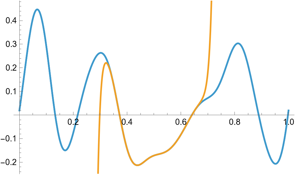
But the Taylor expansion is only applicable to functions that are smooth (i.e., infinitely differentiable). And it is only guaranteed to be a good approximation in a small region around where you are expanding. And you don’t know how close it is to the actual function without having a bunch of extra information (e.g., you need to have a bound on the maximum value of the next derivative over the entire region of interest!). And it is entirely possible that no matter how much of the Taylor expansion you compute, the approximation never improves. And…

You get the picture. There are many practical problems where the Taylor series is completely unworkable. Here’s an example.

Let’s suppose you have a recording of a sound. It is representable as a real-valued function: the input is time and the output is air pressure.

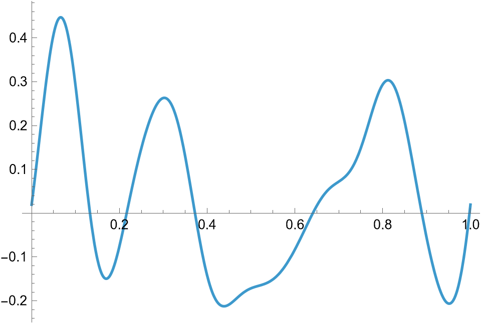
Now, you want to store this on a computer, or even make a copy and send it to your friend. But a computer can only store binary—a sequence of zeros and ones. How do you represent a function with this? You cannot do it exactly, but you can absolutely approximate it—you can even approximate it so precisely that the difference is imperceptible to the ear.

Can I approximate using the Taylor series? Probably not: even if this function is differentiable (which is far from guaranteed!), I don’t have any way of computing that derivative. I can approximate it, of course, by calculating slopes of chords in smaller and smaller intervals. But then I will need to approximate the second derivative the same way, with even more error introduced because it depends on the 1^st derivative. And then I’ll have to look at the third derivative, which is even worse, and…

This is unworkable. Here’s a better approach. Let’s assume for now that this signal is periodic: f(t+T)=f(t) for some T>0. In fact, to make it easier on ourselves, we’ll assume that T=1. (This doesn’t materially change anything, but it is more convenient.) What functions do we know that are periodic? Well, how about sine and cosine? In particular, we might look at sin(2πkx) and cos(2πkx), where k can be any positive integer. These are the pure tones—the physical interpretation is that these are notes, increasing in pitch as k increases. We might guess that if we combine the right notes together, then we can construct our signal. If we only take some finite number of these notes (e.g., those that are in the audible range for humans), then we will get an approximation of our signal. So, we are looking for a linear combination like

\(\sum_{k=0}^\infty \left(a_k \sin(2\pi k x) + b_k \cos(2\pi k x)\right)\)

that will approximate our original function. Here, as is often the case, we can greatly simplify by passing to complex numbers. Specifically, if we remember Euler’s identity that e^it=cos(t)+isin(t), then we can derive that

\(\begin{align*} \cos(t)&=\frac{e^{it}+e^{-it}}{2} \\ \sin(t)&=\frac{e^{it}-e^{-it}}{2i}. \end{align*}\)

If we then plug that into our sum above, we see that we can reduce it to just looking at a sum

\(\sum_{k=-\infty}^\infty c_k e^{2\pi ikt}\)

where the coefficients c_k are now allowed to be complex numbers.

Okay, fair enough, but how can we find these coefficients? Well, observe that

\(\int_0^1 e^{2\pi i k t} \ \text{d}t = \begin{cases} 1 & \text{ if $k=0$} \\ 0 & \text{otherwise}. \end{cases}\)

From this, we might conclude that

\(\int_0^1\sum_{k=-\infty}^\infty c_k e^{2\pi ikt} \ \text{d}t \stackrel{?}{=} \sum_{k=-\infty}^\infty \int_0^1 c_k e^{2\pi ikt} \ \text{d}t = c_0.\)

(There is a reason for the question mark over the equality in the middle there. We’ll get to this later.) Therefore, if

\(f(t)=\sum_{k=-\infty}^\infty c_k e^{2\pi ikt},\)

then we can deduce that

\(c_0=\int_0^1 f(t) \ \text{d}t.\)

Cool: we’ve solved how to determine c₀. How about the other coefficients? We can get them similarly: we just need to generalize the trick, as follows.

\(\int_0^1 e^{2\pi i k t}e^{-2\pi i \ell t} \ \text{d}t = \begin{cases} 1 & \text{ if $k=\ell$} \\ 0 & \text{otherwise} \end{cases}\)

whence

\(\begin{align*} \int_0^1 f(t) e^{-2\pi i \ell} \ \text{d}t &= \int_0^1\sum_{k=-\infty}^\infty c_k e^{2\pi i kt} e^{-2\pi i \ell} \ \text{d}t \\ &\stackrel{?}{=} \sum_{k=-\infty}^\infty\int_0^1 c_k e^{2\pi i kt} e^{-2\pi i \ell} \ \text{d}t \\ &= c_\ell. \end{align*}\)

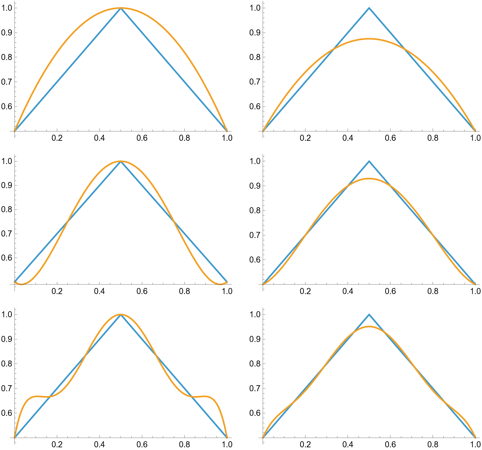
What is nice about this approach? It only requires multiplying by a simple function and integrating—both of those operations are vastly easier to approximate than differentiation. Indeed, here are the results of the first few steps of this process for the function we showed above.

The approximations one gets by only looking at terms with |k|≤0,1,2,3,4,5. The original function is in blue; the approximation is in orange.

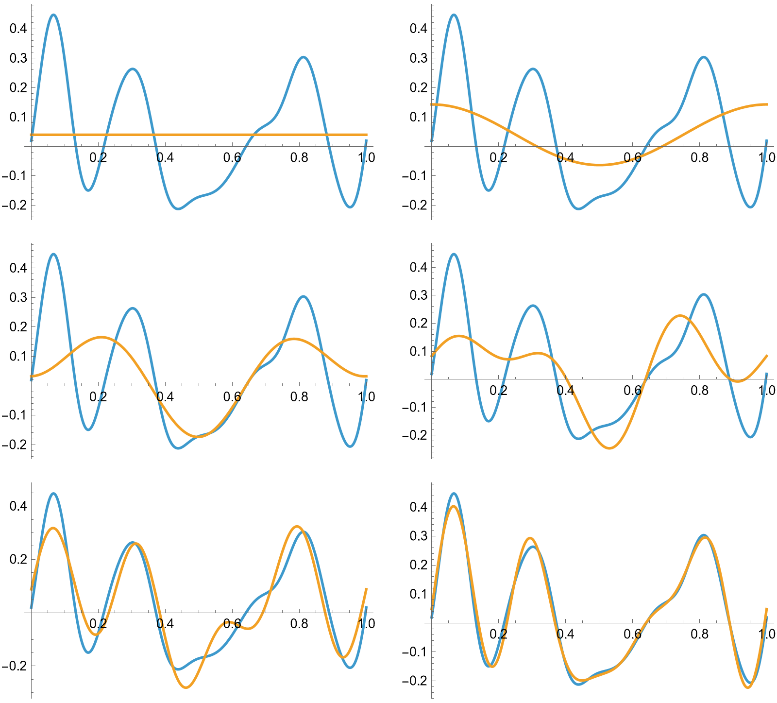
It really does look like everything is nicely converging! And the approximation is quite good over the entire interval, not just around some point. Here’s the Taylor approximation at t=1/2 of order 20, by the way.

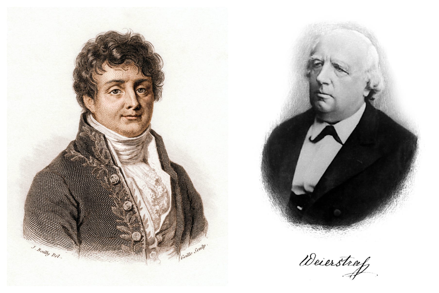
For those who are unaware, we have just discovered the Fourier series. Joseph Fourier originally described this in 1822, motivated in a vaguely similar way: rather than reasoning about sound waves, he was interested in solving the heat equation, which it turns out can be handled in the same way.

Joseph Fourier (left), and Karl Weierstrass (right). We’ll discuss how Weierstrass fits in the picture in a minute.

Except… have we actually handled anything? We’ve created a nice picture for one particular function, but there are all sorts of unanswered questions:

1. How generally does this method work? Does it work for all functions? (This is precisely what Fourier claimed in his original paper!) All periodic functions? All periodic, continuous functions? Something even more restrictive?

2. We would like to say that the infinite sum that we defined converges to our original function. But in what sense? If we’ve only studied calculus, then we know how to say that a sequence of real numbers or perhaps even a sequence of tuples of real numbers converges. But this is something else.

3. Let’s say that we can define what it means for this infinite sum to converge, and we can prove that it does converge to our function. Can we say how well the partial sum approximates the original? What would that even mean?

There’s an obvious answer that we could suggest for question (2): we might say that our sequence of approximations f₁, f₂,… converges to the original function f if for all 0<t<1,

\(\lim_{k\rightarrow \infty} f_k(t) = f(t).\)

That is, f_k converges to f pointwise.

This definition has the benefit of simplicity and essentially nothing else. Pointwise convergence is exceptionally poorly behaved. Let’s illustrate this with an example.

Consider the function

\(f(x)=\begin{cases} 0 & \text{if } 0<\text{mod}_1(x)<1/2 \\ 1 & \text{if } 1/2<\text{mod}_1(x)<1 \\ \frac{1}{2} & \text{otherwise}.\end{cases}\)

(Here, mod₁(x) is x minus the largest integer less than or equal to x.) It is easier to understand from a picture:

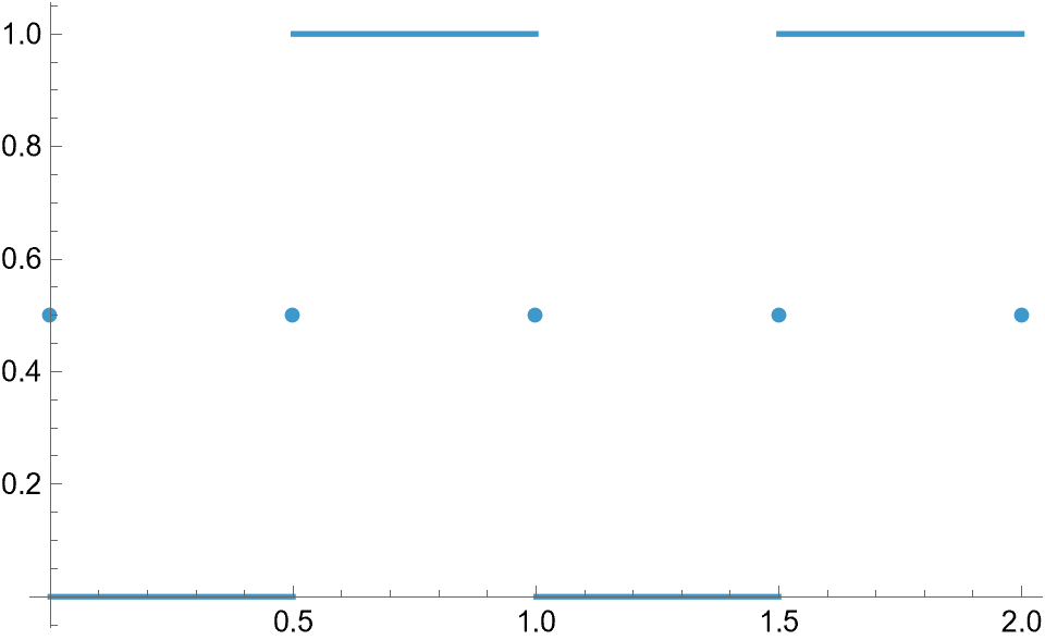
You can think of it as an intermittent signal: it is fully off, then fully on, then fully off, and so on. The switches happen so rapidly that we might as well model it as a sharp jump.

This function is periodic and integrable. It is even continuous most everywhere. It certainly looks like we can take the same approach as before, and indeed, one can compute

\(f(t)=\frac{1}{2}-\frac{2}{\pi}\sum_{k=0}^\infty \frac{\sin(2\pi(2k+1)t)}{2k+1}.\)

Here, the series on the right really does converge pointwise to the function on the left. So far, so good.

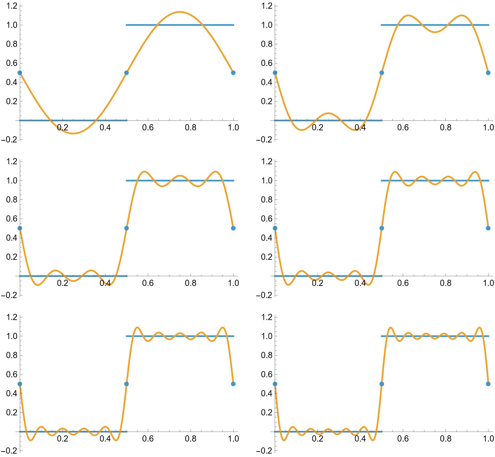
But now, let’s say that we want to differentiate this function—for example, that is precisely what you have to do to solve the heat equation, like Fourier was doing. We expect that differentiation will fail at x=0,1—the function isn’t even continuous there! But there shouldn’t be any problems anywhere else, right? However, if we differentiate the series term by term, we obtain

\(-4\sum_{k=0}^\infty\cos\left(2\pi(1+2k) t\right)\)

which doesn’t converge at all, anywhere other than the discrete set of points where mod₁(t)=1/4, 3/4!

After Fourier published, there was an outpouring of similarly bizarre results from other mathematicians. What he was doing certainly seemed right, but it lead to convergence issues like the above, strange pathological functions that were continuous everywhere but non-differentiable everywhere, and all kinds of other problems.

This forced a huge cultural shift in mathematics. Prior to that point, mathematicians were mostly happy to have intuitive justification for their results¹. Fourier series forced the adoption of rigor—intuition and algebraic calculations were insufficient; there had to be formal definitions and proofs for everything, no matter how seemingly obvious. It is not a coincidence that just a few decades after Fourier’s publication, Weierstrass perfected² the epsilon-delta definition of continuity and finally put calculus on a firm footing. Lebesgue’s development of measure theory was prompted by the fact that it is quite difficult to prove when you can exchange a limit with the Riemann integral, as one does frequently with Fourier series. Cantor began to develop his ideas of cardinality while working with Fourier series—he was thinking about what sort of sets you could reasonably sum over.

Let’s go back to our example of the intermittent signal. There is another problem with it, and a very practical one to boot. Let’s illustrate the next few approximations to our intermittent signal.

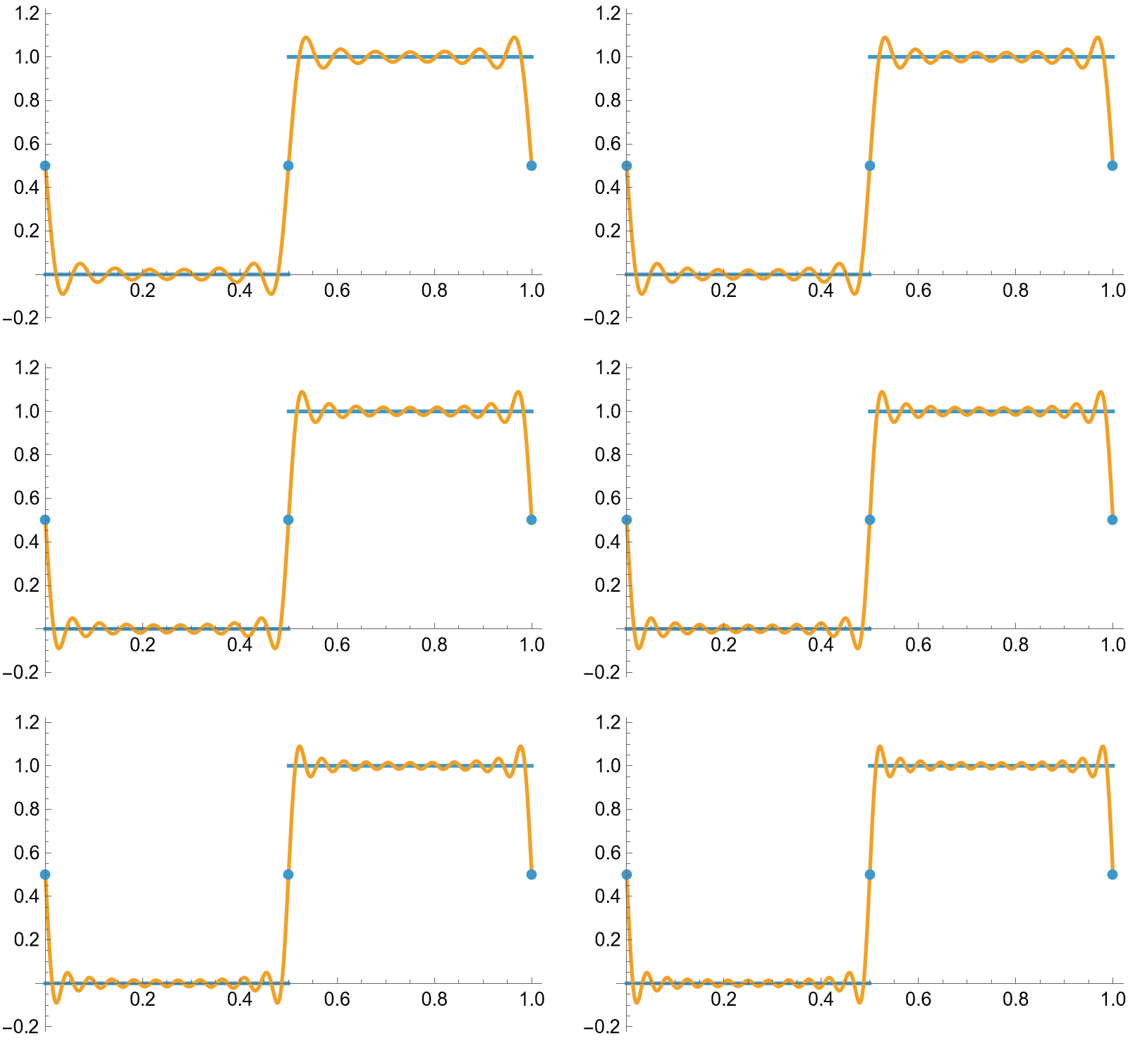
Do you see it? Right around the jump discontinuities, we get weird spikes. These get skinnier and skinnier, but not smaller and smaller.

This is the approximation that one gets with the first hundred terms of the infinite series.

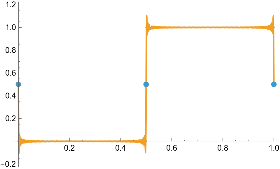
This has a name in the physics community: it is the Gibbs phenomenon. When I was still an undergraduate student in my electromagnetism lab, I was adjusting the dials on the oscilloscope and discovered some kind of bizarre signal that I didn’t expect. I tried to work out what was wrong with my circuit until the professor walked over, took a look, and informed me that this was because of the Gibbs phenomenon. The oscilloscope wasn’t creating a true intermittent signal, but a Fourier approximation, and I had managed to zero in on the part of the signal that was very far from being constant. (Incidentally, this is essentially how the Gibbs phenomenon was originally discovered by experimental physicists—only later did mathematicians explain why it occurs!)

One more thing: in our derivation of the Fourier series, we boldly switched the order of an infinite summation and an integral. Given that we now know that Fourier’s claims about the convergence of Fourier series were a bit suspect, perhaps we should consider whether this is actually justifiable. And, indeed, this is not without issue. Consider the following example:

\(\begin{align*} \int_0^\infty\sum_{n=1}^\infty \left(ne^{-nx}-(n+1)e^{-(n+1)x}\right) \ \text{d}x \\ \sum_{n=1}^\infty \int_0^\infty\left(ne^{-nx}-(n+1)e^{-(n+1)x}\right) \ \text{d}x \end{align*}\)

I leave it as an exercise to the reader to show that the first one is 1, but the second is 0.

Okay. Hopefully, I have convinced you that: 1) these questions are not easy, but 2) well worth answering. But how can we measure how well one function approximates another?

There is no one-size-fits-all solution here. It depends on the particular context: for different types of functions and different specific applications, we might need somewhat different approaches. As a result, rather than developing any singular method, we are going to work on general frameworks in which we can consider such questions; we can then consider particular instances as necessary. This leads us to functional analysis: we want to develop spaces of functions with nice properties.

We’ll start with what is essentially the easiest case: Banach spaces. If there is interest, I may do another post looking at some of the other constructions (e.g., Hilbert spaces and Fréchet spaces).

So, what do we need for our function spaces? Most basically, we need the ability to make sense of linear combinations of functions—that is, we need to consider vector spaces.

---

Definition: A (complex) vector space V is a set together with a binary operation + (which takes two elements in V and returns another in V) such that for all u, v, w in V:

1. Addition is associative: u+(v+w)=(u+v)+w.

2. Addition is commutative: u+v=v+w.

3. There exists an identity (usually called 0): 0+v=v+0=v.

4. Each element u has an inverse (usually called -u): u+-u=-u+u=0.

Additionally, there is a scalar multiplication: an operation ⋅: ℂ×V→V (i.e., it takes a complex number and an element of V, and returns an element of V) such that for all complex numbers c₁, c₂ and elements v, w in V:

1. c₁⋅(v+w)=c₁⋅v+c₁⋅w,

2. c₁⋅(c₂⋅v)=c₁c₂⋅v,

3. (c₁+c₂)⋅v=c₁⋅v+c₂⋅v, and

4. 1⋅v=v.

---

The point is that this is the minimal amount of structure that we need to be able to define (and sensibly work with) finite linear combinations like

\(\sum_{k=0}^n c_k f_k.\)

The trouble is that we need to extend to infinite linear combinations. For that, we need limits.

Now, any student who has gone through real analysis will tell you that as long as you can define a distance function on a space, then you can use that to define limits. And that’s fine, but we want something with a bit more structure than that: whatever distance we dream up should play nicely with the fact that we are working with a vector space. So, for instance, we would probably like it to be true that d(f,g)=d(f+h, g+h): that is, the distance between f and g should be the same as f+h and g+h—we’ve just shifted both over by the same amount.

Well, if we want that to be true, then we really only need to define distance away from 0: after all, d(f, g)=d(f-g, 0), so if we can say how far something is from the origin, that is enough to determine distance everywhere.

What else might we want? Well, we would also like scalar multiplication to play nicely with this distance: in particular, we might ask that multiplying by a scalar scales the distance. By how much? By the magnitude of the scalar, of course! That is, we want d(cf, cg) = |c| d(f, g), where |x+iy|=(x²+y²)^1/2. (That is, it is the usual Euclidean distance.)

Putting it all together and adding the usual requirements for a distance function, we get the following definition.

---

Definition: A normed (complex) vector space is a complex vector space V together with a norm ||⁕||: V→[0, ∞) such that for any v, w in V and complex number c,

1. ||v||=0 if and only if v=0,

2. ||v+w|| ≤ ||v||+||w||, and

3. ||cv|| = |c| ||v||.

We then define the distance between v and w as ||v-w||.

---

The second requirement might look the most puzzling, but it is quite simple: this is just the triangle inequality. That is, the distance from A to B plus the distance from B to C should be no more than the distance from A to C.

This is the geometric picture you should have in mind.

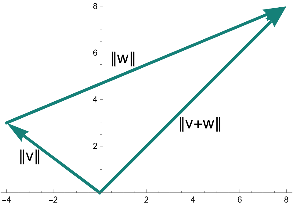
Once you have this, we can define limits without issue, as follows.

---

Definition: Let V be a normed vector space. We say that a sequence f_k in V converges to f in V if and only if

\(\lim_{k\rightarrow\infty} \|f-f_k\| = 0,\)

in which case we write

\(\lim_{k\rightarrow\infty} f_k = f.\)

---

Intuitively, we are just saying that the terms of the sequence are getting closer and closer to f, as measured by our distance function.

There is one last technical restriction that we need, which will be familiar to those with knowledge of real analysis: we need it to be the case that if the terms in the sequence get closer and closer to each other, then they converge to something.

---

Definition: Let V be a normed vector space. A Cauchy sequence in V is a sequence f_k such that

\(\lim_{k\rightarrow\infty}\sup_{m,n\geq k}\left\|f_m-f_n\right\|=0.\)

We say that V is complete if all Cauchy sequences converge.

---

You might remember learning various convergence tests for infinite sums in calculus: all of those are predicated on the fact that the real numbers (or, in our case, the complex numbers) are complete. We don’t need to work out what a series converges to—it is enough to show that the differences in the partial sums get smaller and smaller to be able to conclude that, yes, this converges to something. Trying to work with limits in a space that is not complete is an exercise in frustration. Mercifully, we can always reduce to that case: if a space is incomplete, there is a process by which it can be uniquely expanded into a complete space (appropriately called the completion).

With this groundwork done, the definition of a Banach space is actually really simple.

---

Definition: A Banach space is a complete, normed vector space.³

---

Okay… but what does this have to do with function spaces? This will be easier to understand with some examples.

First and foremost, consider ℂⁿ. This is the collection of complex vectors (c₁,c₂,…c_n). (Here, as always, ℂ represents the set of complex numbers.) There are a variety of norms that we could give this⁴, but the most common is

\(\|(c_1,c_2,\ldots,c_n)\|_2=\sqrt{|c_1|^2+|c_2|^2+\ldots+|c_n|^2}.\)

This is just the standard Euclidean distance. With this choice⁵, ℂⁿ is a Banach space.

Now, you might protest here that ℂⁿ doesn’t seem like it has anything to do with function spaces. Not so! There are multiple ways to interpret this as a space of functions. Here are two:

1. Let X be a set with n elements. Consider the collection of functions X→ℂ. How can I represent such a thing? Well, I associate a complex number to each of the n elements of X… which is just the same as a vector in ℂⁿ!

2. Consider the collection of complex polynomials of degree n-1. Each such polynomial c₁+c₂X+…c_nX^n-1 is uniquely defined by the coefficients… which, again, is a vector in ℂⁿ.

The norm we have given is not necessarily the best—there are others that we could consider that might be better suited for a particular problem. For instance, the Manhattan norm is

\(\|(c_1,c_2,\ldots,c_n)\|_1=|c_1|+|c_2|+\ldots+|c_n|.\)

The name is inspired by how it is to travel in Manhattan or any other grid-based city: there are many paths of equivalent length, but all that matters is how many blocks one needs to travel in one direction (north-south, usually) and in the other (east-west).

Here we have two points, and some paths between them. But all of those paths will have length 4+3=7.

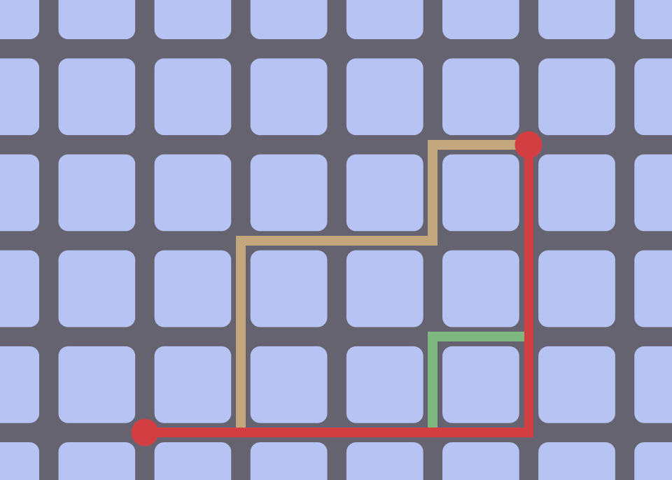
We might also want to consider the sup-norm:

\(\|(c_1,c_2,\ldots,c_n)\|_\infty=\max\left(|c_1|,|c_2|,\ldots,|c_n|\right).\)

In general, for any p≥1, we have the p-norm:

\(\|(c_1,\ldots,c_n)\|_p=\left(|c_1|^p+\ldots+|c_n|^p\right)^{1/p}.\)

You can think of the sup-norm as being the limit as p→∞.

Emboldened by this success, let’s try to generalize it: we could take an arbitrary set X and consider the collection of functions X→ℂ. This is a complex vector space… but is it a normed space?

We could try to define

\(\|f\|_p := \left(\sum_{x\in X} |f(x)|^p\right)^{1/p}.\)

This is just the same p-norm, except that instead of summing over finitely many elements, we are potentially summing over infinitely many (everything in X, specifically)… and that is a bit of a problem, because f(x)=1 identically is a perfectly fine function, but the corresponding sum does not converge if X is infinite.

How to fix it? Well, we could take inspiration from how the space of polynomials works: rather than looking at all functions X→ℂ, we instead look only at those functions that take non-zero values for some finite collection of inputs. (If we take an arbitrary polynomial c₁+c₂X+c₃X²+…, we might not know the degree, but we know that c_k=0 if k is big enough.) Then the infinite sum above is not a problem (because it is really a finite sum, in disguise), so we get a normed vector space.

But is it complete? No! Consider the functions f_k: ℤ→ℂ (here, as always, ℤ represents the integers) defined by

\(f_k(n)=\begin{cases} 1 & \text{if $n = 0$} \\ \frac{1}{n} & \text{if $0<|n|\leq k$} \\ 0 & \text{if $|n| > k$}. \end{cases}\)

These are all in our space. It is easy to check that they define a Cauchy sequence with respect to the 2-norm:

\(\begin{align*} \|f_m-f_n\|_2&=\sum_{\ell=m+1}^n \frac{2}{\ell^2} \\ &\leq\int_{m+1}^\infty \frac{2}{x^2} \ \text{d}x \\ &= \frac{2}{m+1} \rightarrow 0. \end{align*}\)

But this sequence doesn’t converge to anything in our space! With that said, it is quite clear what it “should” converge to:

\(f(n)=\begin{cases} 1 & \text{if $n = 0$} \\ \frac{1}{n} & \text{otherwise}. \end{cases}\)

This might not be in our space, but we can see that

\(\|f\|_2=\sqrt{1+2\sum_{n=1}^\infty \frac{1}{n^2}}<\infty.\)

This inspires the following definition.

---

Definition: Let X be any set, and let p≥1. We define ℓ^p(X) to be the set of all functions f: X→ℂ such that

\(\sum_{x\in X} |f(x)|^p < \infty.\)

We also define a norm on this space via

\(\|f\|_2 := \left(\sum_{x\in X} |f(x)|^p\right)^{1/p}.\)

Similarly, we define ℓ^∞(X) to be the set of bounded functions f: X→ℂ, and we define a norm on this space via

\(\|f\|_\infty = \sup_{x\in X}|f|.\)

---

These are now bona fide Banach spaces!

Unfortunately, they work quite well for discrete spaces (like ℤ), and not so well for anything else. For example, for any p<∞, any function in ℓ^p([0,1]) will have to be zero almost everywhere. This, for instance, means that we cannot meaningfully talk about Fourier series.

Let’s look at the only exception: p=∞. The entire space of all bounded functions f: [0,1]→ℂ is a bit too big—it includes all kinds of random scatterings of points. But it has a subspace which is entirely reasonable: C([0,1]), which is the collection of continuous functions f: [0,1]→ℂ. This is quite clearly a vector space, and we can give it the same norm as for the parent space ℓ^∞([0,1]). But is it complete?

Another way to ask that question is: if we take any sequence of continuous functions f_k: [0,1]→ℂ that converge to f: [0,1]→ℂ with respect to the sup-norm, must f be continuous? Yes: this is the uniform limit theorem, commonly taught in real analysis. Ergo, C([0,1]) together with the sup-norm is a Banach space.

This space is important enough that most real analysis classes will spend a significant amount of time considering it and its properties. For instance, the Stone-Weierstrass theorem tells you that for any f in C([0,1]), there exists a sequence of polynomials p_k that will converge to f.

An example: the first few terms of a sequence of polynomials that converge to a function with a triangular graph.

Actually, both the uniform limit theorem and Stone-Weierstrass tell you much more: for example, if you take any closed and bounded subset X of ℝⁿ (here ℝ is the collection of real numbers), then C(X) will be a Banach space and any element in it can be approximated by a sequence of (multivariate) polynomials.

This, incidentally, tells us something interesting about Fourier series. Choose any continuous, periodic function f: [0,1]→ℂ. This can, equivalently, be viewed as the collection of continuous, complex-valued, periodic functions on the unit circle 𝕊¹ inside ℝ². From the above, we know that it can be approximated by a sequence of polynomials in two variables X and Y—let’s write it as

\(p_k=\sum_{m=0}^\infty\sum_{n=0}^\infty c_{k,m,n} X^m Y^n,\)

where c_k,m,n=0 for all but finitely many m and n. But what are X and Y here? Since we are on the unit circle, we can parametrize as X=cos(2πt) and Y=sin(2πt). Or, if we prefer, we can rewrite this in terms of e^2πit. Expanding out and rewriting everything, we suddenly discover that

\(p_k=\sum_{n=-\infty}^\infty d_{k,n} e^{2\pi i n t},\)

where d_k,n=0 for all but finitely many n. And, therefore,

\(f(t)=\lim_{k\rightarrow\infty}\sum_{n=-\infty}^\infty d_{n,k}e^{2\pi i n t}.\)

This is almost the Fourier series expansion! If we can justify switching the order of the summation and the limit, then it will be exactly the Fourier series—we’ll just replace each of the d_n,k’s with their limit… assuming that such a thing exists.

Justifying this swap is actually a bit subtle—in fact, it isn’t true in general! It is entirely possible to have a continuous, periodic function such that the Fourier series doesn’t converge to it even pointwise, let alone in ℓ^∞.⁶ Let’s set our sights much, much lower and simply prove that the coefficients d_n,k do actually converge to something. This will already require a bit of non-trivial theory.

Let’s return to our ℓ^p spaces where p<∞. We want to find something like it, but which isn’t forced to be zero almost everywhere.

Well… why not just replace the sum with an integral? That is, we could define

\(\|f\|_p:=\left(\int_0^1 |f(t)|^p \ \text{d}t\right)^{1/p}.\)

For what sort of functions could we define this? Well, based on what we did before, we might suggest taking the collection of continuous functions f: [0,1]→ℂ. The resulting space will certainly be a vector space, and you can check that the p-norm above will make it a normed space. But is it complete? Or, put another way, is the p-norm limit of a sequence of continuous functions continuous?

No. Not in general—let’s build a counter-example.

Let f_k be a function that linearly interpolates between 0 and 1, as follows: if t<1/2-1/n, then it is 0; if t>1/2+1/n, then it is 1; between these two ranges, it is (2+(2n-1)x)/4, which is just the connecting straight line. A picture is easier to understand:

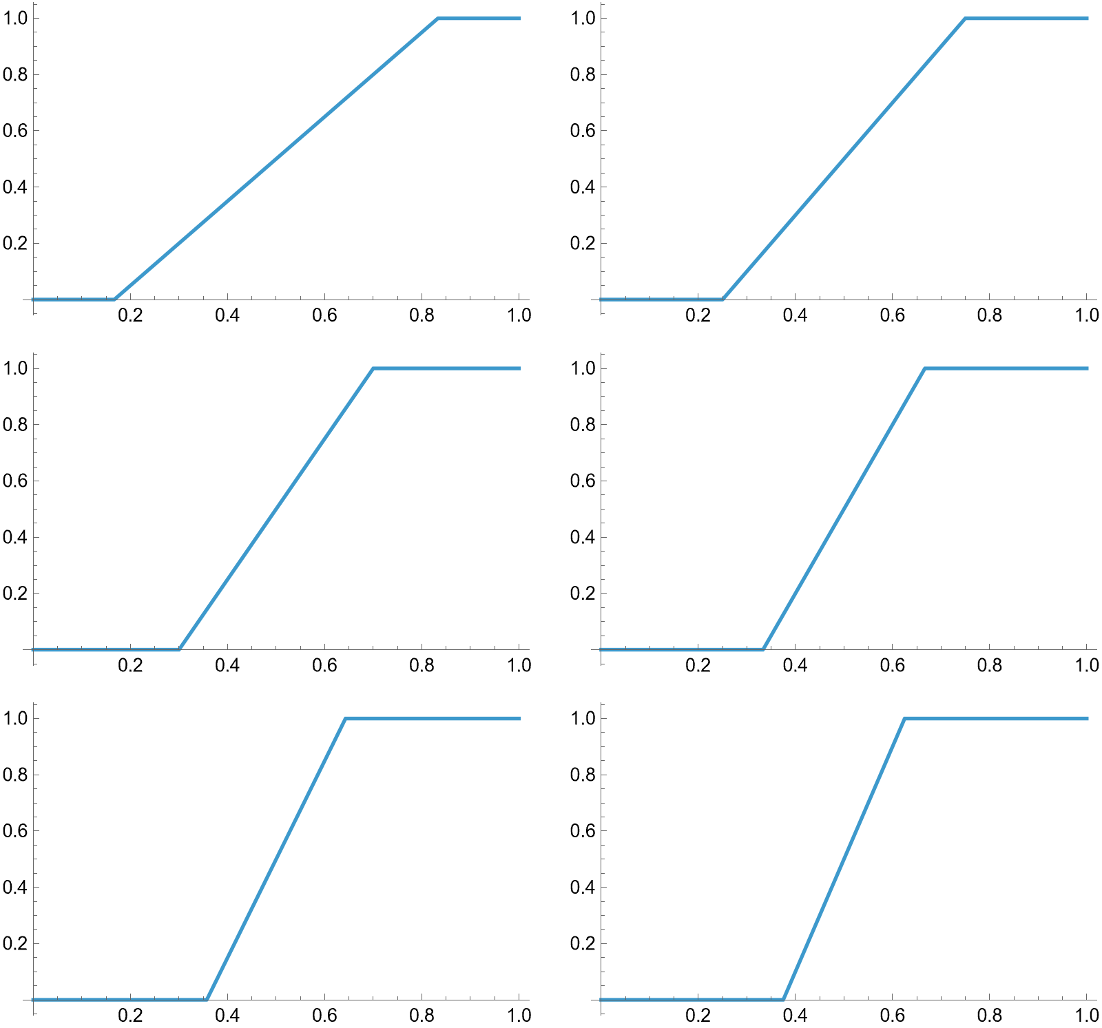
Is this a Cauchy sequence with respect to the 2-norm? Yes—the distance between f_m and f_n will be less than the area under the interpolating line for the smaller of m and n. Without loss of generality, that is m, which means that the distance is bounded above by 1/m, which will go to 0.

What does it converge to? Certainly not any continuous function! If you stare it, you might guess that it converges to the intermittent signal that we looked at earlier… and that is exactly right!

So our space is incomplete, and we need to throw on functions like the intermittent signal to make it complete. We might guess, based on what we saw for the ℓ^p spaces, that the right thing is to consider all functions for which

\(\int_0^1 |f(t)|^p \ \text{d}t <\infty.\)

This is almost right, but there is a wrinkle. Suppose I have a function that is zero everywhere except at some finite number of places. Then

\(\int_0^1 |f(t)|^p \ \text{d}t =0.\)

Therefore, the p-norm of this function is 0. But, remember, an important part of the definition of a normed space is that ||f||=0 if and only if f=0!

There is an easy resolution to this: consider two functions to be the same if they agree almost everywhere.

---

Definition: We say that two integrable functions f, g: [0,1]→ℂ are equivalent if

\(\int_0^1 |f(t)-g(t)| \ \text{d}t = 0.\)

For any p≥1, L^p([0,1]) is the space of functions f such that

\(\int_0^1 |f(t)|^p \ \text{d}t<\infty,\)

considered up to equivalence. (Meaning, we consider two functions in this space to be the same if they are equivalent.) We then define a p-norm

\(\|f\|_p:=\left(\int_0^1 |f(t)|^p \ \text{d}t\right)^{1/p}.\)

Similarly, L^∞([0,1]) is the space of all essentially bounded functions, considered up to equivalence—that is, a function is in this space if one of the function that it is equivalent to is bounded. We define a norm by

\(\|f\|_\infty = \text{ess sup}_{0\leq x\leq 1}|f(x)|.\)

This is the essential supremum, which we might define thus: it is the smallest value of the supremum taken among all functions equivalent to f.⁷

---

These are, once again, Banach spaces. More importantly, we can state a very nice convergence theorem in terms of these Banach spaces.

---

Theorem: (Duality of L^p Spaces) Choose any 1≤p<∞. Let 1≤q≤∞ be such that 1/p+1/q=1. (We match 1 to ∞ here, and vice versa). Then L^q([0,1]) is the dual of L^p([0,1]): every continuous, linear function Φ: L^p([0,1])→ℂ is of the form

\(\Phi(f)=\int_0^1 f(t) g(t) \ \text{d}t\)

for some g in L^q([0,1]), and vice versa.

---

The main ingredients in the proof are the dominated convergence theorem from measure theory, and Hölder’s inequality, which is typically one of the first things that one proves in a functional analysis class. (Hölder's inequality is also crucial for proving that L^p([0,1]) is a Banach space in the first place.)

In any case, remember, we showed that

\(f(t)=\lim_{k\rightarrow\infty}\sum_{n=-\infty}^\infty d_{n,k}e^{2\pi i n t}.\)

The limit was with respect to the ℓ^∞ norm, which we might recognize as being the same as the L^∞ norm in this case. Furthermore, observe that if f_k→f with respect to the L^∞ norm on [0, 1], then actually f_k→f with respect to the L^p norm. Here’s why: choose a k sufficiently large so that ess sup(f-f_k) < ε. Then

\(\begin{align*} \|f-f_k\|_p &= \left(\int_0^1 |f(t)-f_k(t)|^p \ \text{d}t\right)^{1/p} \\ &\leq \left(\int_0^1 \epsilon^p \ \text{d}t\right)^{1/p} = \epsilon. \end{align*}\)

What does that tell us? Well, consider the functions

\(\Phi_m(f) := \int_0^1 f(t) e^{-2\pi im t} \ \text{d}t.\)

These are continuous, linear functions L^p([0,1])→ℂ. Why? Because e^-2πimt is in L^q([0,1]), which is the dual! Since they are continuous and linear, we may conclude that

\(\begin{align*} \Phi_m(f)&=\lim_{k\rightarrow\infty}\sum_{n=-\infty}^\infty d_{n,k}\Phi_m\left(e^{2\pi i n t}\right)\\ &=\lim_{k\rightarrow\infty}d_{m,k}. \end{align*}\)

So, yes, the limit exists—it is precisely the expected Fourier coefficient!

1. Someone will no doubt complain that I am underplaying, say, the Greeks’ reliance on proofs. But the proofs of ancient Greeks weren’t altogether rigorous by modern standards: they relied crucially on the diagrams that came with them. Algebra was closer to being rigorous, except where infinite series were concerned, and that is where all the meat is here.

2. I’m being careful with my wording, because some epsilon-delta arguments occurred earlier: Bolzano had already considered it, but his work was unknown until after his death, and Cauchy also did some work along these lines, but not always so formally. (E.g., Cauchy argued at one point that the pointwise limit of continuous functions is continuous, which is simply not true.)

3. Lest I be accused of misinforming the reader: although I have chosen to define Banach spaces exclusively over the complex numbers, one can do the same construction with reals. But real Banach spaces are used somewhat less frequently than complex Banach spaces.

4. Although, for many applications it really doesn’t matter which one we choose—they are all equivalent in some sense!

5. Well, with any choice (see the previous footnote)!

6. However, it has to converge pointwise almost everywhere. This can be deduced from the theory of Banach spaces.

7. This is more natural to state in the language of measure theory, but I am trying to keep the prerequisites as light as possible.